Authors:
(1) Yujie Hu, Department of Geography, University of Florida, Gainesville, FL 32611 and UF Informatics Institute, University of Florida, Gainesville, FL 32611;
(2) Changzhen Wang, Department of Geography & Anthropology, Louisiana State University, Baton Rouge, LA 70803;
(3) Ruiyang Li, Children’s Environmental Health Initiative, Rice University, Houston, TX 77005;
(4)Fahui Wang, Department of Geography & Anthropology, Louisiana State University, Baton Rouge, LA 70803.
Table of Links
Concluding comments, Acknowledgement and References
Results
Based on the 2010 block population data, population weighted centroids for the 32,840 ZIP codes in the U.S are created. Together with the two network datasets of different road levels, they are fed into Algorithm 1. This process results in a massive OD cost matrix of 1,078,432,760 records, each of which consists of estimation of drive time and distance for a ZIP code pair. It takes about 76 hours for Algorithm 1 to compute and export the national ZIP-to-ZIP time matrix, and the breakdowns are: Level 1 consumes 6 hours, Level 2 60 hours, and Level 3 10 hours.
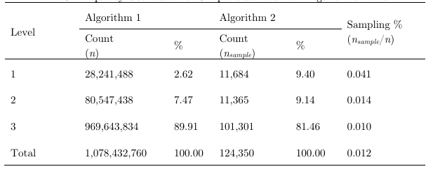
Algorithm 2 is implemented on a randomly-sampled subset of OD pairs derived from Algorithm 1. Given the free usage constraints discussed previously, Algorithm 2 is run to collect Google drive times over a period of four months. It finally gathers 124,350 (nsample) valid ZIP-to-ZIP trips, which are associated with 32,478 unique ZIP codes (about 99% of the national 32,840 ZIP codes). Each trip includes Google’s estimates of drive time and distance. Table 3 lists the frequency distribution of OD trips derived from Algorithms 1 and 2. The sampling intensity for the short-range trips (Level 1) is about triple those medium-range trips (Level 2) and quadruple those long-range trips (Level 3).
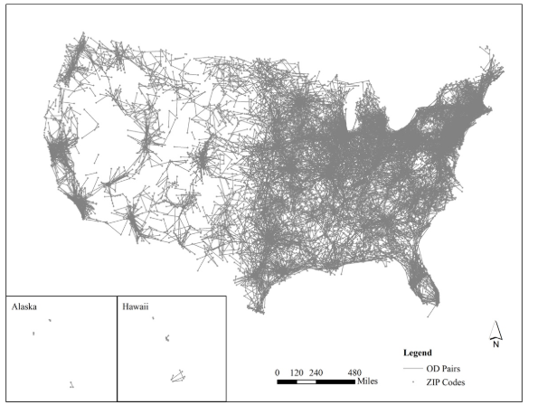
Oversampling shorter trips is to enhance their representation and ensure the quality of subsequent interpolation for greater interests in acquiring shorter-range travel times. Figure 3 shows sampled ZIP code pairs of Level 1.
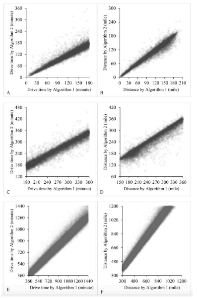
Figures 4A, 4C, and 4E (and 4B, 4D, 4F) plot drive times (distances) estimated by Algorithm 1 against times (distances) by Algorithm 2 at Level 1, 2 and 3, respectively. Only the data points within 24 hours (1,200 miles, or 1,931 km) for Level 3 are shown. Clearly, the pattern is largely consistent between the two algorithms for ZIP code pairs across the three levels. A few observations merit discussion. It is obvious in Figures 4A and 4C that Algorithm 1 tends to underestimate travel times. One likely cause for this trend is the omission of congestion in Algorithm 1. Interestingly, such a trend of downward estimates is also observed in distance measurements in Figures 4B and 4F. This is because the distances returned by Algorithm 2 are simply the lengths in mileage of those quickest routes in terms of drive times, which are commonly through highways. Therefore, distances measured by Algorithm 1—the “shortest” routes in terms of mileage—are consistently lower than the values estimated by Algorithm 2. The exact fitting power of each needs to be examined by regression.
Corresponding to each of the three levels in Algorithm 1, a regression is run to infer the relationship between Google drive times by Algorithm 2 (dependent variable) and Algorithm 1 drive times (independent variable). Results are summarized in Table 4. It shows that Algorithm 1 times explain the variation in the matched Google times by 91 percent at Level 1, 93 percent at Level 2, and 96 percent at Level 3. Table 4 also reports the results for regression models on distance measures from the two algorithms, with the R2 = 0.95, 0.93, and 0.99 for Levels 1, 2 and 3, respectively. The higher fitting powers by the travel distance models than the drive time ones are due to the uncertainty in traffic congestion effect on drive time measurement. As travel distances are not used as often as drive times in measuring spatial impedance, our discussion focused on drive time
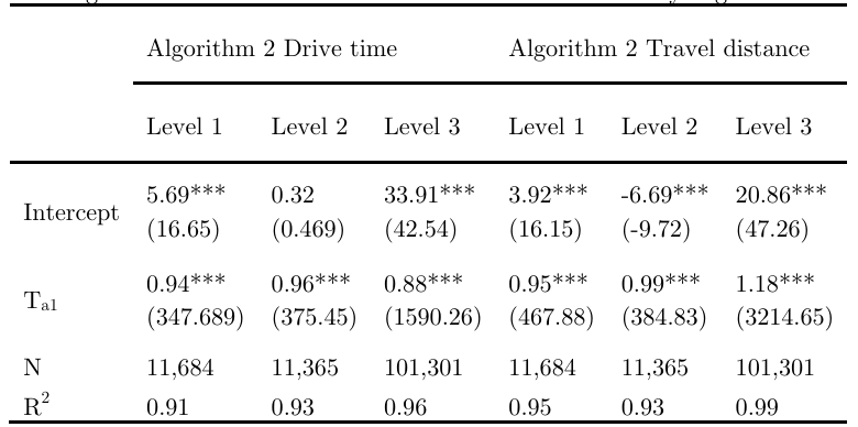
Note: Ta1 represents Algorithm 1 derived drive times and distances, and N denotes the number of observations.
***Significant at the 0.001 level.
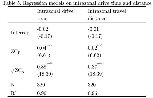
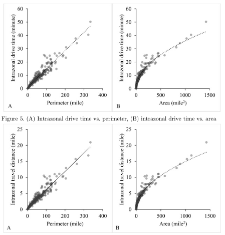
area Originally designed by the United States Postal Service (USPS), ZIP code is a fivedigit number corresponding to address points in the U.S., and such data have never been released by the USPS for public access. It is, therefore, not an areal unit where a ZIP code has a specified physical boundary. For the sake of spatial analysis, many entities have attempted to delineate ZIP code areas, such as the ZCTAs by the U.S. Census (Khan et al., 2019). Our recent experience in using this drive time matrix indicates that some USPS ZIP codes are not included in the ZCTAs data. Most of those missing ZIP codes have no associated area such as post office box ZIP codes and single site ZIP codes (government, building, or large volume customer). One may use the following algorithm to interpolate the drive times on corresponding missing OD pairs:
- For drive time between a missing ZIP code (say, origin) and a known ZIP code (say, destination): identify the 3 nearest known ZIP codes from the missing ZIP code, locate the 3 drive times between each of the 3 nearby known ZIP codes (origin) and the known ZIP (destination) from the provided matrix, and use their average drive time as the one between the missing ZIP code and the known ZIP code.
- For drive time between two missing ZIP codes: identify the 3 nearest known ZIP codes from the origin ZIP code and also the 3 nearest known ZIP codes from the destination ZIP code, locate the corresponding 9 drive times between each of the 3 nearby origins and each of the 3 nearby destinations from the provided OD cost matrix, and use their average drive time as the one between the two missing ZIP codes.
The above proposition assumes that the location of a missing ZIP code can be approximated by the average of its three nearest ZIP codes.
This paper is available on arxiv under CC BY 4.0 DEED license.

